Unlocking the Power of Predictive Models and Regression Analysis

In today’s data-driven world, understanding and harnessing the power of predictive models is crucial across various industries, including medical physics. This article will guide you through the fundamental concepts of Artificial Intelligence (AI), Machine Learning (ML), and Data Science, before diving deep into predictive models, with a special focus on regression analysis. We’ll explore how these technologies are differentiated, yet interconnected, and walk through a practical case study to illustrate their application.

Differentiating AI, Machine Learning, and Data Science

These terms are often used interchangeably, but they represent distinct concepts within the realm of data and intelligence:

• Artificial Intelligence (AI): This is the broadest field, encompassing techniques that enable machines to simulate human-like thinking and problem-solving. It’s about creating intelligent agents that perceive their environment and take actions that maximize their chance of achieving their goals.
• Machine Learning (ML): A subset of AI, ML focuses on algorithms that allow systems to learn from data without explicit programming. This learning often involves identifying patterns and making predictions, which is central to predictive modeling.
• Data Science: This interdisciplinary field involves extracting knowledge and insights from structured and unstructured data. It combines statistics, programming, and domain expertise to prepare, analyze, and interpret data, forming the foundational bedrock for building effective ML models.

The Five Steps of Data Science

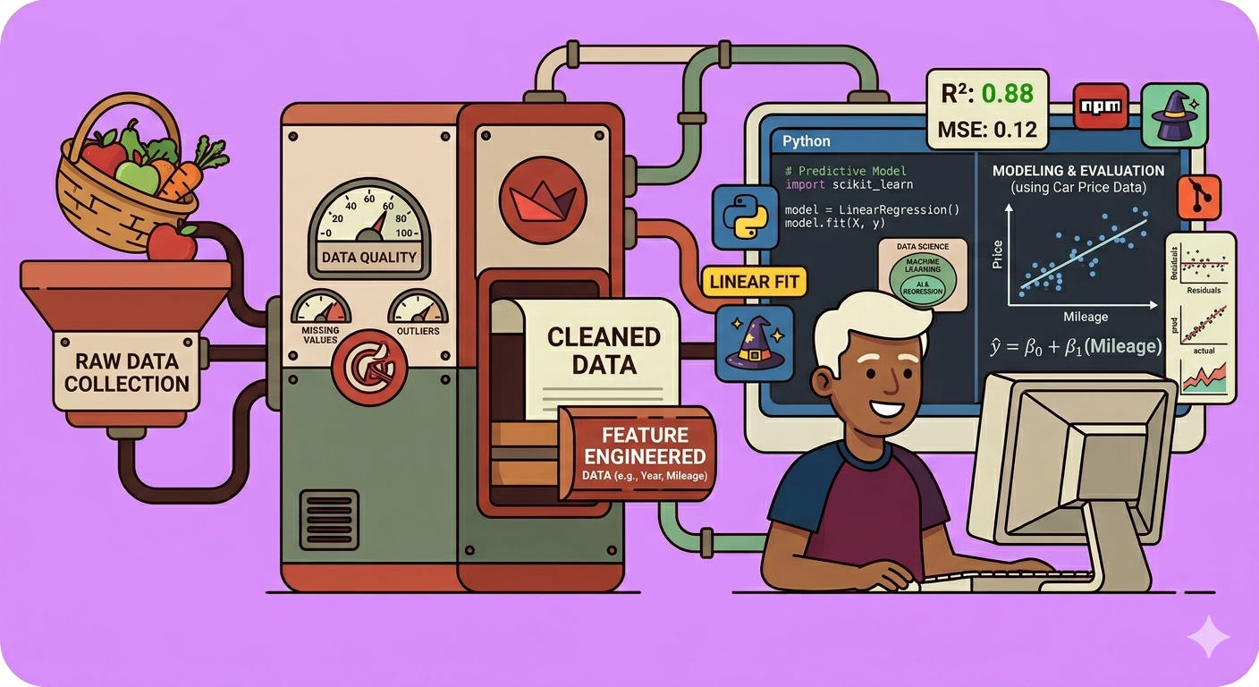
Data Science is a systematic process crucial for preparing data for predictive modeling:

1. Data Collection: Gathering raw, often unstructured data from various sources.
2. Data Cleaning: Transforming raw data into a structured and interpretable format. This involves handling outliers (extreme values that can bias results) and missing values.
3. Data Exploration: Understanding the characteristics of the data, identifying relationships between variables, and determining how they can be appropriately used.
4. Modeling: Feeding the cleaned and explored data into a chosen algorithm to begin the learning process.
5. Visualization: Presenting the outcomes of the model in an interpretable way, and assessing their reliability. This step often leads back to earlier stages for refinement.

To illustrate these steps, consider a basket of fruits and vegetables. From this, you can collect raw data like the type of item, quantity, weight, price, and freshness. Data cleaning would involve categorizing items (e.g., fruit vs. vegetable) and distinguishing between categorical (non-countable, like ‘type’) and continuous (countable, like ‘weight’) variables. Exploration would involve discovering relationships, such as how price might increase with weight or type. These initial steps are vital before any predictive modeling can begin.

Understanding Predictive Models

Predictive models use historical data to forecast future outcomes. They are essential for data-driven decision-making across many industries – from predicting weather to stock prices. Building a predictive model typically involves four stages:

1. Data Preparation: As discussed, this involves cleaning and structuring your data.
2. Model Selection: Choosing the appropriate algorithm based on the nature of your data and the desired outcome.
3. Training: Feeding your prepared dataset to the chosen model so it can learn patterns and relationships.
4. Evaluation: Assessing the model’s performance and accuracy using unseen data.

Algorithm Selection: The Heart of Predictive Modeling

Selecting the right algorithm is critical. Various types of predictive algorithms exist, each with its own advantages and limitations:

• Linear Regression: For data with a linear relationship between variables, predicting a continuous numerical value.
• Logistic Regression: For predicting a probability or a binary outcome (e.g., yes/no, true/false).
• Decision Trees, Random Forests, Gradient Boosting: Powerful algorithms for both classification and regression, often used for complex, non-linear relationships.
• Support Vector Machines (SVM): Effective for classification and regression tasks, particularly in high-dimensional spaces.
• K-Nearest Neighbors (KNN): A non-parametric algorithm used for classification and regression based on proximity to nearest data points.
• Neural Networks (Deep Learning): Advanced algorithms, especially suited for complex pattern recognition tasks like image and speech processing.
• Polynomial Regression: Used when the relationship between variables is curvilinear.
• Ridge Regression & Lasso Regression: Regularization techniques designed to prevent overfitting, particularly useful when dealing with many correlated features.

Deep Dive into Linear Regression

Linear regression is a foundational predictive model used when variables have a linear relationship. For instance, in our fruit basket example, the price of an apple might increase linearly with its weight.

The core idea is to find a “best-fit line” that describes the relationship between a dependent variable (the outcome you want to predict, e.g., price) and one or more independent variables (the factors influencing the outcome, e.g., weight).

The equation of a simple linear regression line is typically represented as: \(y = m x + c + \epsilon\) where:

• $y$ is the dependent variable.
• $x$ is the independent variable.
• $m$ is the slope of the line, indicating how much $y$ changes for a unit change in $x$.
• $c$ is the y-intercept, the value of $y$ when $x$ is zero.
• $\epsilon$ (epsilon) represents the error, which is the difference between the actual value ($y$) and the predicted value ($\hat{y}$).

The model iteratively adjusts the slope ($m$) and intercept ($c$) to minimize this error. This iterative minimization process is known as optimization.

Training and Evaluating a Linear Regression Model

Step 1: Data Splitting Before training, the dataset is split into two parts:

• Training Data: Used to teach the model and identify patterns.
• Testing Data: Unseen data used to evaluate how well the trained model performs on new, independent data. A common split is 70% for training and 30% for testing.

Step 2: Model Evaluation Metrics After training, the model’s performance is crucial to assess. Several metrics are used for this:

• Mean Squared Error (MSE): Calculates the average of the squared differences between predicted and actual values. Higher MSE indicates a larger difference.
• Root Mean Squared Error (RMSE): The square root of MSE, providing an error metric in the same units as the dependent variable, making it more interpretable.
• Mean Absolute Error (MAE): The average of the absolute differences between predicted and actual values, less sensitive to outliers than MSE.
• R-squared ($R^2$): Also known as the coefficient of determination, it represents the proportion of the variance in the dependent variable that can be predicted from the independent variable(s). A higher R-squared value (closer to 1) indicates a better fit.
• Adjusted R-squared: A modified version of R-squared that adjusts for the number of predictors in the model. It helps assess whether adding more independent variables actually improves the model’s predictive power or simply increases its complexity without real benefit.

Case Study: Predicting Car Prices with Linear Regression

To demonstrate the application of linear regression, let’s consider a case study of predicting car prices using a dataset of 50,000 retail car listings.

Workflow:

1. Data Loading: Load the raw dataset, which contains various features like vehicle type, seller name, price, year of registration, power, mileage, etc., and potentially outliers or missing values.
2. Column Extraction: Select only the relevant columns that are likely to influence the car’s price, such as price, year of registration, month of registration, power, and mileage.
3. Data Cleaning: This is a critical step:
   • Remove duplicate entries to prevent bias.
   • Handle missing values (e.g., by imputation or removal).
   • Filter out unreasonable or invalid data (e.g., cars registered in the future, or cars with extremely low or high prices/mileage that are likely errors).
4. Feature Engineering: Enhance the dataset to create more meaningful features:
   • Convert month of registration into a fractional year and calculate the age of the car (which directly impacts price more than the month/year alone).
   • Derive power per kilometer from power and mileage to capture a combined efficiency metric.
   • Apply log transformation to the price to handle its wide range and ensure better model stability.
   • Drop unused original columns (e.g., original year of registration if age is now used).
   • Create dummy variables for categorical features (e.g., fuel type, brand) to convert them into a numerical format suitable for regression.
5. Data Splitting: Divide the processed data into training (e.g., 70%) and testing (e.g., 30%) sets.
6. Model Training: Train a linear regression model using a library like scikit-learn in Python on the training data.
7. Model Evaluation: Use the test data to evaluate the trained model using metrics like RMSE and R-squared.
   • In the presented example, an RMSE of 11942 for the training set and 9652 for the test set was observed. This shows that the model’s predictions vary from actual values by approximately these amounts. The difference indicates that while the model has learned, there’s still room for improvement, likely by including more features or refining existing ones. A lower RMSE on the test set compared to the training set can sometimes indicate good generalization, but significant differences might also point to underfitting if the training error is high.
8. Prediction: Use the final trained model to predict car prices based on new input parameters.

The resulting equation for price prediction in this case study looked like: \(\log(\text{price}) = 8.728 + (0.0001 \times \text{age}) + (0.00005 \times \text{power}) + (-0.000001 \times \text{mileage}) + \dots\) where 8.728 is the intercept, and the coefficients reflect how each feature influences the log of the price.

Real-World Applications in Medical Physics

Predictive models, especially those built on robust data science principles, have numerous applications in medical physics:

• Predictive Maintenance of Radiotherapy Equipment: Predicting when a linear accelerator (linac) might require maintenance based on historical performance data, dose output, and error logs, thereby minimizing downtime.
• Patient Outcome Prediction: Using patient-specific data, treatment parameters, and tumor characteristics to predict treatment response or potential side effects in radiotherapy.
• Dosimetry Quality Assurance (QA): Predicting dose distributions based on patient CT scans and treatment plans, or predicting the accuracy of dose delivery based on machine parameters.
• Optimizing Treatment Planning: Developing models that can suggest optimal beam arrangements or dose fractionation based on previous successful treatments and patient-specific factors.
• Image Reconstruction and Analysis: Predicting features in medical images or improving image quality based on limited input data.

Conclusion

AI, ML, and Data Science are powerful tools that, when understood and applied correctly, can revolutionize various fields. Predictive models, particularly regression analysis, allow us to leverage historical data to make informed forecasts. The key takeaway is that even complex AI systems start with fundamental steps like data preparation and cleaning. By mastering these basics, we can build sophisticated models that drive significant advancements, even in specialized fields like medical physics.